What if? Causal inference through counterfactual reasoning in PyMC
Unravel the mysteries of counterfactual reasoning in PyMC and Bayesian inference. This post illuminates how to predict the number of deaths before the onset of COVID-19 and how to forecast the number of deaths if COVID-19 never happened. A must-read for those interested in causal inference!

Have you started to hear people talk about causal inference and wanted to know more? Have you looked into causal inference but been daunted by unfamiliar concepts, notation, and software packages? Do you wonder what the relationship between causal inference and Bayesian modeling is? Fear not! While the field of causal reasoning is complex and nuanced, we can make meaningful inroads pretty easily.
This first post on causal reasoning will demonstrate that it is accessible and that we can use a bunch of Bayesian concepts that we are already familiar with. Not only that, we'll show how this can be done in Python and PyMC.
Counterfactual inference: asking what if?
Imagine you had just finished a $1/4 million advertising campaign and your company wants to know what the impact of that was. Maybe they will ask "Did the campaign work?" "How much revenue did the campaign generate?" "How many customers did the campaign acquire?"
These are questions about causal effects of the campaign, and questions like this can be answered by considering specific counterfactual, or "what if" questions. For example, "How many more sales did we get, compared to a hypothetical scenario where we did not run the campaign?" In order to answer questions like this, we could calculate excess sales caused by the advertising campaign by comparing the actual number of sales to the expected number of sales in a hypothetical timeline where we did not run the campaign.
This post will cover how we can do counterfactual inference, and how we can do this in PyMC, using the example of calculating excess deaths due to COVID-19 (and all related effects, such as changes in availability of medical care). This approach could be applied to many other domains of course, including estimating excess sales due to a marketing campaign, or improvement in school achievement given an educational intervention.
Excess deaths in England and Wales
Excess deaths are defined as:
$$\text{Excess deaths} = \text{Reported Deaths} - \text{Expected Deaths}$$
where the number of reported deaths are a (potentially noisy or lagged) measurement of a real objectively observable aspect of the world. However expected deaths is a counterfactual concept - it is not observable in our timeline. This represents the number of reported deaths that we would expect if COVID-19 had not occurred.
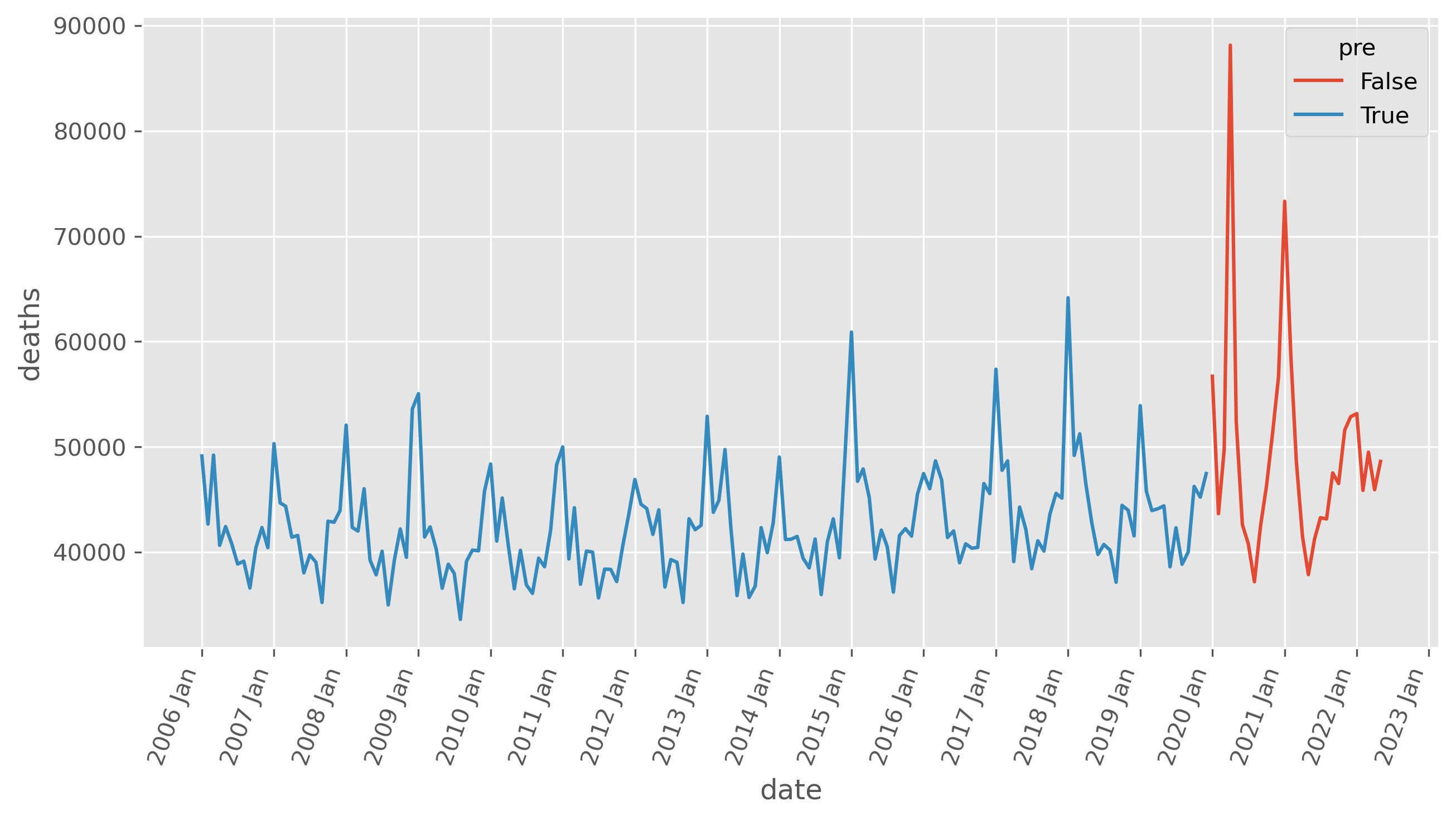
Let's take a look at the data we have. We have the total reported deaths per month in England and Wales, going back a good few years and up to the time of writing.
A Bayesian causal model
Now that we have a feel for the data, we are going to consider a reasonably simple model of the number of reported deaths, as shown in the causal DAG below.

This model considers causal effects of:
- Time: To be clear, we are using time as a proxy variable to capture an increasing number of susceptible (i.e. older) individuals over time, because of the particular population pyramid in England and Wales.
- Month: To capture the clear seasonality we can see in the data. Bear in mind that we are not claiming that the abstract concept of a month kills people, but we are using this as a proxy variable for a whole host of seasonal factors.
- Temperature: Which is also seasonal and has a clear causal pathway in which it can impact the number of deaths. We are using monthly average temperatures across the UK, but it may be that looking at temperature extremes have a clearer causal influence.
Our end goal here is to calculate excess deaths. Therefore we want to build a model focussing on explaining expected deaths before COVID-19. So even though we know for a fact that many people died from COVID-19 (both directly, and indirectly) we do not include COVID-19 as a predictor, neither as a binary before/after onset, nor the prevalence of cases. Instead, we use our model to predict expected deaths in the post-COVID period (without giving it any information about COVID-19), then subtract the number of reported deaths to arrive at our target: excess deaths.
In addition to defining the causal structure in the DAG above, we need to specify the relationships (i.e. the edges, or arrows). Specifically, this means we need to define
$$ \text{deaths}_t = f(\text{time}_t, \text{month}_t, \text{temp}_t) $$ where there are $t=1, \ldots, T$ monthly observations.
There are many different modelling approaches we could take here to define $f$, but for simplicity we will treat this as a linear regression model. So we could consider a model like this:
$$ f(\text{time}_t, \text{month}_t, \text{temp}_t) = \beta_0 + \beta_1 \text{time}_t + \beta_2 \text{temp}_t + \vec{s}[\text{month}_t] $$ where $\vec{s}$ is a vector of 12 monthly deflection parameters.
Building a Bayesian model in PyMC
The good news is that if you already know how to write simple Bayesian models, then you can probably follow this:
$$ \begin{aligned} \beta_0 & \sim \text{Normal}(40000, 10000)\\ \beta_1 & \sim \text{Normal}_+(0, 50)\\ \beta_2 & \sim \text{Normal}(0, 200)\\ s_m & \sim \text{Normal}(0, 3000) \quad \text{for}~ m = 1, 2, \ldots, 12\\ \mu_t & = \beta_0 + \beta_1 \cdot \text{time} + \beta_2 \cdot \text{temperature}_t + \vec{s}[\text{month}_t]\\ \sigma & \sim \text{HalfNormal}(2000)\\ \text{deaths}_t & \sim \text{Normal}_+(\mu, \sigma)\\ \end{aligned} $$
The core of the model here is the linear regression equation which defines $\mu$ above. The rest just defines the likelihood (our prior over the data) and our priors over the model parameters $\beta$. We don't show the PyMC code here, but see the full notebook for all the implementation details.
A nice feature of PyMC is that we can generate plots of the DAG, see below. These are clearly more involved than the simple causal DAG we have above - but these are in fact doing much the same thing. It is simply that the PyMC DAG is more detailed, including nodes for the parameters and intermediate computations (i.e. $\mu$).
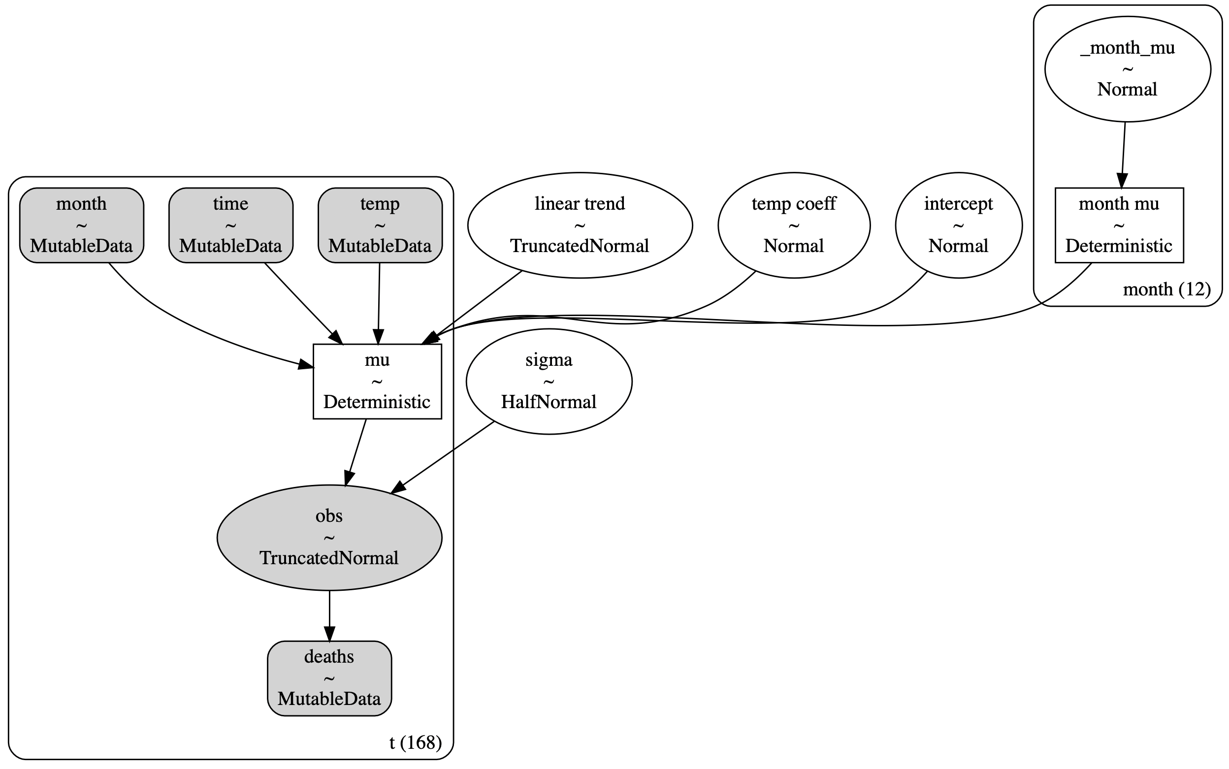
What we've done here with our PyMC model is to describe the full joint distribution $P(\text{time, month, temp}, \vec{\beta}, \vec{s}, \sigma)$.
Using the model
Prior predictive distribution
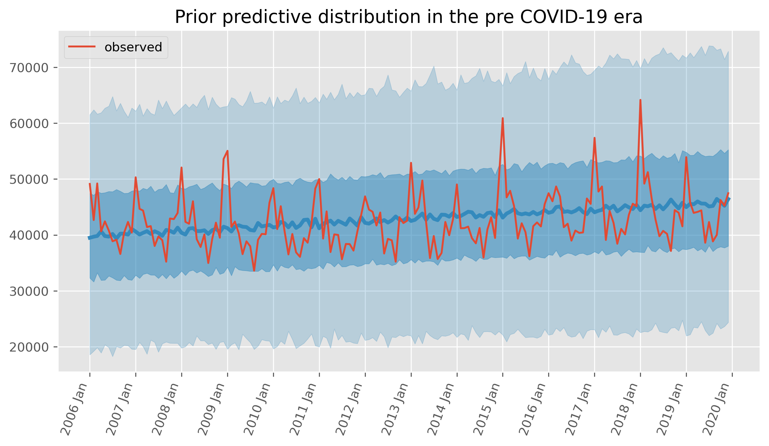
We query what the model would predict before having observed any data. We can do this in PyMC, sampling from the prior predictive distribution $P(\text{deaths}|\vec{\beta}, \vec{s}, \sigma)$.
Inferring a posterior distribution over parameters
We can use PyMC in order to generate MCMC samples which approximate a distribution over parameters, conditioned on the data:
$$ P(\vec{\beta}, \vec{s}, \sigma | \text{time}, \text{month}, \text{temp}) $$
where $\text{time}$, $\text{month}$, $\text{temp}$ are vectors of observations before the onset of COVID-19.
Let's do causal inference!
Firstly, we want to use the model in order to get the models predictions (technically retrodictions) about the number of deaths we observed before the onset of COVID-19. This is an important step - if the model does not do a good job of predicting the observed deaths before the onset then why would we expect it to make good counterfactual predictions of future deaths in the counterfactual world of no COVID-19?
Second, we can use the famous do-operator. This is the crux of the lesson here on counterfactual inference - we are querying what the model forecasts if we were to surgically intervene in some variables. In this case, we will make an intervention and set the time, month, and temp variables equal to the post COVID-19 era. In other words, we are doing a counterfactual forecasting, querying what we believe the deaths would have been from January 2020 onwards in the case where COVID-19 never happened. This query can be expressed as:
$$ P(\text{deaths} | \vec{\beta}, \vec{s}, \sigma, \text{do} (\text{time}=\mathbf{t}, \text{months}=\mathbf{m} , \text{temp}=\mathbf{temp})) $$
where $\mathbf{t}$, $\mathbf{m}$, and $\mathbf{temp}$ are vectors of values of time indexes, months, and temperatures in the forecast time period we are interested in. Practically, we do this in PyMC using the pm.set_data() function which allows us to change the value of our input variables to now represent those from the post-COVID-19 period. That way, our predictions generated by pm.sample_posterior_predictive() will be our expected deaths in our period of interest.
with model:
    # do-operator
    pm.set_data({"month": month_post, "time": time_post, "temp": temp_post})
    # sample from this out of sample posterior predictive distribution
    counterfactual = pm.sample_posterior_predictive(idata, var_names=["obs"])
where month_post, time_post, and temp_post are vectors of the months, time indexes and temperatures in the post COVID-19 onset period we are considering.
So how did we do?
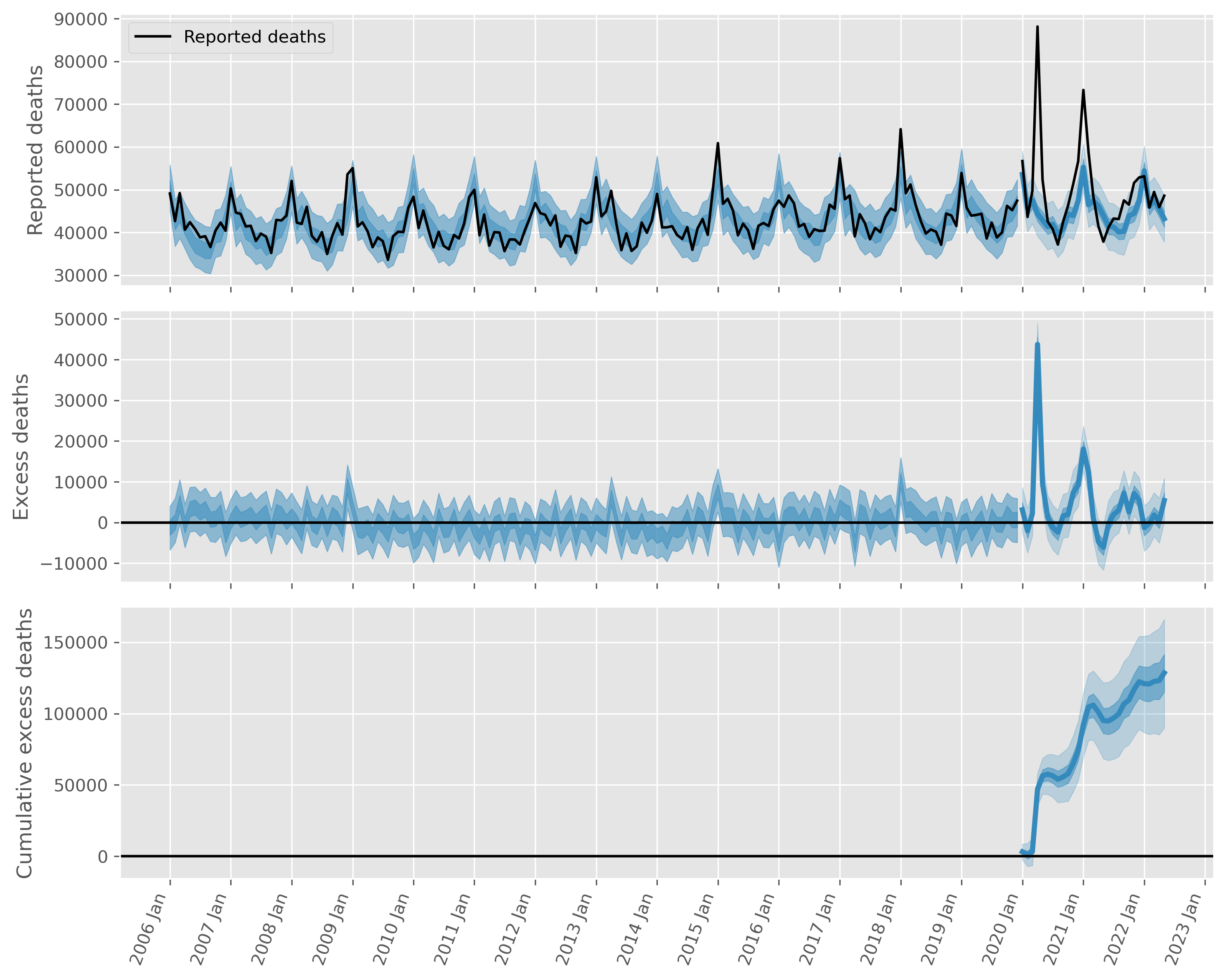
First, looking at the pre COVID-19 era (before January 2020), we can see that the model does a reasonable job of accounting for the actual observed pre COVID-19 deaths. Second, we can see in the post COVID-19 era, the observed number of deaths is meaningfully higher than our counterfactual expected number of deaths had COVID-19 not happened. We can then use the formula above to calculate the excess deaths (middle panel), and also cumulate to estimate the distribution of cumulative excess deaths (lower panel).
And there we have it! We used our existing knowledge about Bayesian inference and outlined how we can approach counterfactual reasoning in PyMC. We've taken a small but important step into the world of causal inference!
Resources
See the full notebook for all the implementation detail that shows how to implement the material covered in this post.
Acknowledgements
Thanks to Eric Ma for his causality notebooks which were particularly useful in preparing this post.
Work with PyMC Labs
If you are interested in seeing what we at PyMC Labs can do for you, then please email info@pymc-labs.com. We work with companies at a variety of scales and with varying levels of existing modeling capacity. We also run corporate workshop training events and can provide sessions ranging from introduction to Bayes to more advanced topics.